|
|
|
equalization |
 This window models the channel shape and corrects the global
frequency response by applying an inverse curve. This is known as
"equalizing the channel" which is quite similar to how an audio equalizer
might be used to correct the frequency response of the room / speaker
combination in a home theater or recording studio environment. Note that
this equalizer works only in the frequency domain; it does not correct for
multipath, so it is not yet a true equalizer in the modem sense.
This window models the channel shape and corrects the global
frequency response by applying an inverse curve. This is known as
"equalizing the channel" which is quite similar to how an audio equalizer
might be used to correct the frequency response of the room / speaker
combination in a home theater or recording studio environment. Note that
this equalizer works only in the frequency domain; it does not correct for
multipath, so it is not yet a true equalizer in the modem sense.
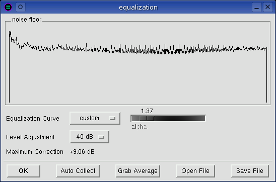
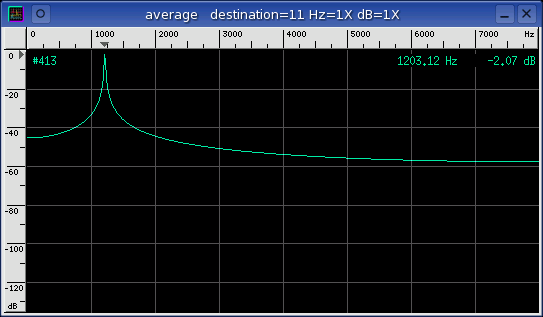
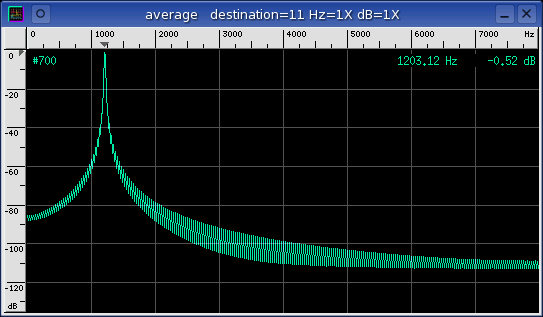
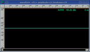
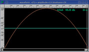
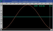
noise floor
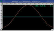
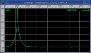
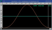
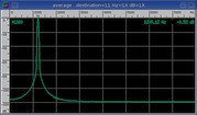
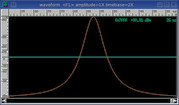
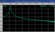
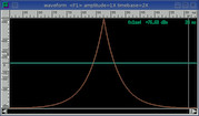
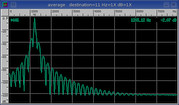
Noise floor is a pictorial representation of the channel shape. The
inverse of this frequency response is the equalization curve. Like the
Average or Spectrum windows, this is a frequency vs dB display.
 Equalization Curve
Choose a preset equalization curve, build a custom curve, or turn off
equalization with the flat setting. Note that custom
equalization curves are automatically saved on program exit and loaded next
time baudline is started.
alpha
This slider is only sensitive when the 1 / f ^ alpha equalization curve
is set. Alpha represents the slope in -dB / octave. Note that
alpha=1.0 is proper 1 / f noise, and alpha=3.0 is pink noise.
Level Adjustment
Since the goal of equalization is to make the frequency response as flat as
possible, noise floors that have strong tones will result in large
corrections. This will push the spectral energy up which could result in
clamping at the 0 dB level and it might impair visualization resolution or
scaling. This control reduces the post equalization spectral levels so
that strongly equalized signals can be brought back into a usable zone.
Maximum Correction
This displays in dB the maximum value of the current equalization curve.
Auto Collect
There are two modes of operation - record and
pause. In record mode, the custom curve is cleared, average collection
begins, and the name of the button changes to "Stop Collect." The noise
floor displays the equalization curve as it collects. The longer duration
the spectrum is collected, the smoother it gets, and the more accurately it
represents the true channel shape. Hitting the Stop Collect
button halts the average spectra collection, inverts the curve, and applies
it as the new custom curve. In pause mode, the custom curve is cleared,
the selected Spectrogram data (or ALL data if none) is average collected,
and the frequency response is applied as the new custom curve. Note
that both of these modes of operation are equivalent to manually collecting
data in the average window and then
hitting the Grab Average button which is described below.
Grab Average
Copy the current Average destination spectrum and paste it here as the
custom equalization curve.
Open/Save File
Load a new custom equalization curve from a file. Or save the currently
selected equalization curve to a specific file. The file format is the
same as is used in the average window.
The format is two column (Hz, dB) ASCII text which can be plotted with xgraph
or gnuplot.
|
|
|
|
progress bar |
 This window pops up every time a lengthy calculation is being performed.
It displays the current status from 0% to 100% and it has a Stop button for
halting the current calculation.
This window pops up every time a lengthy calculation is being performed.
It displays the current status from 0% to 100% and it has a Stop button for
halting the current calculation.
This window can pop up from a paste done in the
average or
histogram windows, from an Auto Collect
operation done in the equalization
window, or from a stdout paste operation.
|
|
|
|
transform size |
 This selects the size of the Fast Fourier Transform
(FFT) that is used internally. Transform
sizes range from 128 up to 65536 bins in power of 2 increments. There are
benefits to using both larger and smaller FFT sizes. Larger FFT's have a
finer frequency resolution and a higher SNR (this means they are better
at extracting weak signals). Smaller FFT's use less CPU resources and
they have a finer time resolution (they blur time variant signals
less).
This selects the size of the Fast Fourier Transform
(FFT) that is used internally. Transform
sizes range from 128 up to 65536 bins in power of 2 increments. There are
benefits to using both larger and smaller FFT sizes. Larger FFT's have a
finer frequency resolution and a higher SNR (this means they are better
at extracting weak signals). Smaller FFT's use less CPU resources and
they have a finer time resolution (they blur time variant signals
less).
Note that the number of frequency bins is the value of half of the transform
size. So a 2048 point transform generates 1024 pixels width of frequency
resolution. If the spectral windows are resized smaller than this value,
the "extra" information is just discarded not rescaled unless a Hz zoom
factor is selected.
The bin resolution (Hz / bin) which is how many Hz are in each FFT bin can be
found by looking in the
popdown options section of the
Drift Integrator window. The bin resolution is a function of both
transform size and sample rate.
|
|
|
|
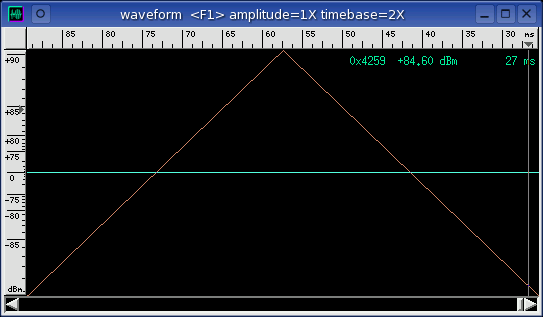
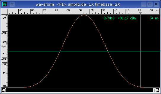
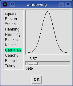
windowing |
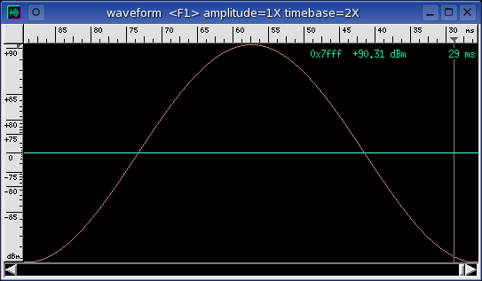
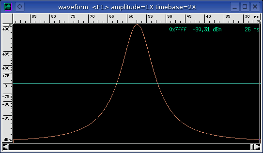
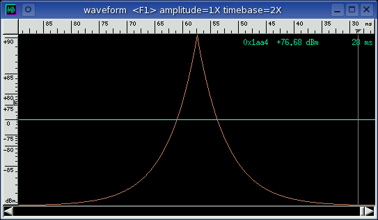
 The windowing function is applied by multiplication to a signal slice before
the Fourier transform is done. Windowing is important because it reduces
wraparound leakage. It widens the lobe width while it increases the time
resolution detail.
The windowing function is applied by multiplication to a signal slice before
the Fourier transform is done. Windowing is important because it reduces
wraparound leakage. It widens the lobe width while it increases the time
resolution detail.
 Note that the Fourier and Correlation
transforms use the windowing
functions while the Raster and Histogram transforms ignore it.
Note that the Fourier and Correlation
transforms use the windowing
functions while the Raster and Histogram transforms ignore it.
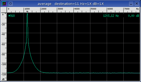
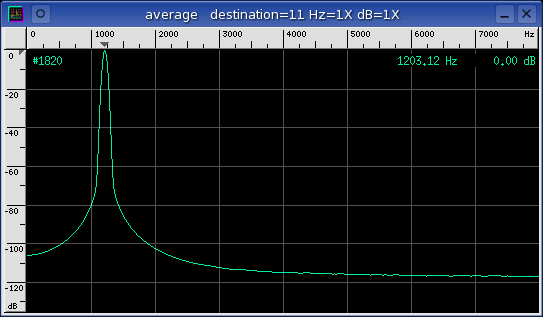
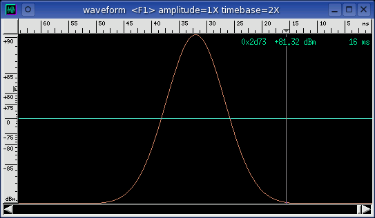
Windowing function characteristics can vary dramatically. Some windows
are designed for general purpose work while others are very specialized.
Several of the windows even have an adjustable beta variable that can modify
the windowing shape.
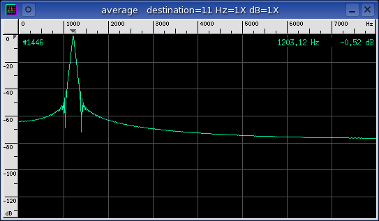
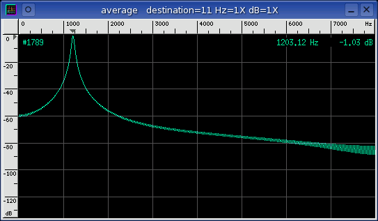
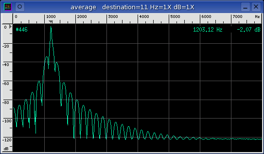
The Hanning, Blackman (default), and Kaiser (beta=14) windows are good for
general spectral analysis work. The Welch and Gaussian windows have
special feature extraction abilities that are optimized respectively for weak
signal and short duration (enhanced time-domain resolution) uses. See the
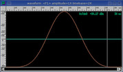
windowing gallery below for details and notes about each specific window:

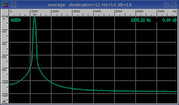
 Square
|
Formula:
|
1.
|
|
Overlap:
|
50%
|
|
SINAD:
|
57.6 dB
|
|
Notes:
|
Flat top.
The square window has the narrowest lobe width at top center but it also has a
lot of wrap leakage and wide skirts.
|
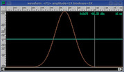
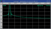
 Parzen
|
Formula:
|
1. - abs(x / N - 1.)
|
|
Overlap:
|
29.5%
|
|
SINAD:
|
88.9 dB
|
|
Notes:
|
Triangle shape.
Oscillating side bands.
Also known as the Bartlett window.
|
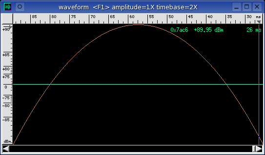
 Welch
Welch
|
Formula:
|
1. - (x / N - 1.)^2
|
|
Overlap:
|
34.8%
|
|
SINAD:
|
82.8 dB
|
|
Notes:
|
Parabolic shape.
Maximum sensitivity for weak signal work.
|
 Hanning
|
Formula:
|
0.5 - 0.5 * cos(pi * x / N)
|
|
Overlap:
|
26.6%
|
|
SINAD:
|
96.6 dB
|
|
Notes:
|
Cosine shape.
Good for general purpose use.
Also known as the von Hann window.
|
 Hamming
|
Formula:
|
0.54 - 0.46 * cos(pi * x / N)
|
|
Overlap:
|
28.7%
|
|
SINAD:
|
35.1 dB
|
|
Notes:
|
Raised cosine shape introduces minor leakage.
|
 Blackman
|
Formula:
|
0.42 - 0.5 * cos(pi * x / N) + 0.08 * cos(2 * pi * x / N)
|
|
Overlap:
|
22.5%
|
|
SINAD:
|
95.9 dB
|
|
Notes:
|
Default.
Thinner version of Hanning window.
Good for general purpose use.
|
 Kaiser
|
Formula:
|
bessel(beta * sqrt(1. - (1. - x / N)^2)) / bessel(beta)
|
|
Beta:
|
14.
|
|
Overlap:
|
17.8%
|
|
SINAD:
|
95.6 dB
|
|
Notes:
|
A beta of 14 is good for general purpose use.
Thinner and adjustable beta version of Blackman window.
Increase beta for enhanced time-domain resolution.
|
 Gaussian
|
Formula:
|
e^(-0.5 * (beta * (1. - x * N))^2)
|
|
Beta:
|
6.
|
|
Overlap:
|
11.3%
|
|
SINAD:
|
96.0 dB
|
|
Notes:
|
Thinner version of Kaiser window.
Increased beta range for enhanced time-domain resolution.
Pull out the individual symbols of an FSK
modem at the highest beta settings.
|
 Cauchy
|
Formula:
|
1. / (1. + (beta * (1. - x * N))^2)
|
|
Beta:
|
6.
|
|
Overlap:
|
14.3%
|
|
SINAD:
|
71.0 dB
|
|
Notes:
|
Slightly rounded exponential.
Increased beta range for enhanced time-domain resolution.
|
 Poisson
|
Formula:
|
e^(beta * (x / N - 1.))
|
|
Beta:
|
6.
|
|
Overlap:
|
11.5%
|
|
SINAD:
|
81.4 dB
|
|
Notes:
|
Pointy exponential.
Increased beta range for enhanced time-domain resolution.
|
 Tukey
Tukey
|
Formula:
|
0.5 - 0.5 * cos(pi / beta * x / N)
|
|
Beta:
|
6.
|
|
Overlap:
|
46.3%
|
|
SINAD:
|
26.3 dB
|
|
Notes:
|
Flat top with cosine tapered edges.
Identical to Hanning window at max beta.
|
The overlap percent was calculated using the 100%
Optimum Slide Size value from the
Drift Integrator window.
The SINAD measurement was made with a 0
dB digital amplitude 1209.10 Hz sine wave. Note that SINAD is basically
equivalent to SNR for these sine windowing test measurements.
|
|
|
|
|