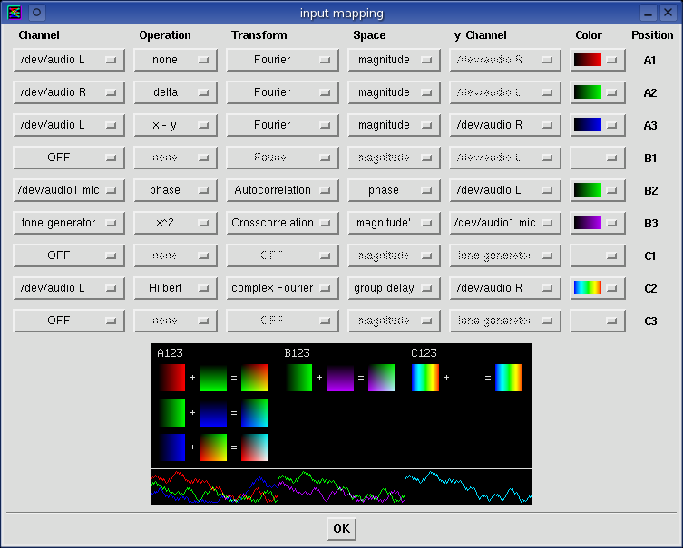
The input channel mapping window makes baudline highly configurable.
The mapping of processing operations, transforms, spaces, colors, and
routing positions of every channel can be completely controlled.
The input channel mapping window makes baudline highly configurable.
The mapping of processing operations, transforms, spaces, colors, and
routing positions of every channel can be completely controlled.
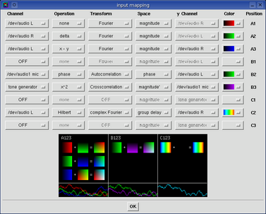
Click the thumbnail below for a larger image.
Now this is a very complicated looking window,
but fortunately most users will never have to use it because baudline
automatically configures itself depending on how things are setup in the
input devices window. The general
auto configuration defaults are: pack every channel as tightly as possible, no
operations, Fourier transform, magnitude display, and a unique, and a
constructively summable color ramp.
Note that unlike the input devices window, all the controls here are post
buffer, which means they are nondestructive and changing them will
retroactively affect all the data in the buffer. Changes can be made
while either recording, paused, or playing.
 Channel
Only enabled channels from the input devices window are visible in this
option menu. The channel selected here will be processed by the following
corresponding rules and then displayed at the indicated row position (A1 C2
...). Enabled input devices can be chosen multiple times or not at all if
desired. Think of the Channel column as simply a means of mapping
any particular input device to any of the 9 possible display
positions.
 Operation
These time-domain operations allow the user to program baudline to perform
some simple yet powerful channel and inter-channel analyses. They work
on the input channel sample data and they range from simple arithmetic to more
complex DSP operations. Some operations are dual channel and require a
second channel (see the y Channel).
Like all the other channel mapping rules in this window, these operations
do not permanently change the buffered data and they are completely
reversible. Note that operations are performed prior to the file saving
action. For example: a stereo file can be converted to a mono file by
using the x + y operation.
| operation |
description |
| none |
no modification (default) |
| -x |
invert, 180° phase shift |
| | x | |
absolute value |
| 1 / x |
reciprocal |
| sqrt |
square root, negative values retain sign |
| x^2 |
square |
| x^3 |
cube |
| x^4 |
quad power |
| log |
logarithm, negative values retain sign |
| clip |
discard all quantization bits except for sign bit |
| delta |
difference coding, X(n) - X(n+1) |
| | delta | |
absolute value of the delta operation |
| -Hz |
negative frequency, flip frequency axis |
| Hilbert |
90° phase shift |
| bits |
convert sample to bits |
| bit reverse |
flip bit order, MSB becomes LSB |
| flip endian |
swap bytes, little endian <---> big endian |
| |
|
| x + y |
dual channel, addition |
| x - y |
dual channel, subtraction |
| x * y |
dual channel, multiplication |
| x / y |
dual channel, division |
| x % y |
dual channel, modulus |
| xor |
dual channel, bitwise exclusive OR |
| magnitude |
dual channel, sqrt(x^2 + y^2) |
| phase |
dual channel, atan2(x, y) |
Note that the majority of these time-domain operations also perform scaling
so that sample overflow is avoided. For example; when the variables x and
y are the same the x + y operation will equal x due to scaling.
 Transform
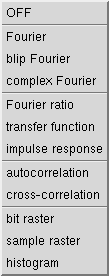
A transform is a mathematical operation that converts between domains.
The end product of the transform is displayed in baudline's spectrogram and
spectrum based windows. Time domain based samples are the typical
transform input but frequency domain samples are an option with specialized
hardware. Other input domains are also possible. Below are
descriptions of the different transforms with accompanying spectrogram snippet
images of a sine wave.

The Fourier transform (FFT) converts a time
domain signal to the frequency domain. The Fourier transform
option is the default and it takes a real time domain signal as input.
The complex Fourier transform performs the Fourier transform on a
complex signal which is represented by two inputs: an in-phase (I) component
from the Channel menu, and a quadrature (Q) component from the y Channel
menu. For information on automatic complex Fourier mapping see the
-quadrature command line option.
The Fourier ratio takes the difference between two Fourier transforms
of two different input channels.

The blip Fourier transform utilizes a blind phase locking algorithm
built on a new analysis primitive called the blip(let) to enhance the spectral
display in both magnitude and phase spaces. This does two valuable
things. First, the spectral resolution is improved in the
magnitude space which is ideal for observing amplitude beating while deep
zooming down to the sample level. Second, spinning phase is now locked which
allows the phase space to contain visibly useful information. A focus
parameter in the process menu allows for fine tuning the algorithm on a signal
by space by zoom basis. For more information see the
blip Fourier preview
and
blip
BPSK demodulation blog posts.

The transfer function is a dual channel transform that is useful for
observing the relationship between the input and output of a system.
It is a linear mapping of the Laplace transform of the input X(f) to the
output Y(f) in the formula Y(f) = H(f) * X(f) where H(f) is the transfer
function and the "*" operator is convolution. Another way of looking
at H(f) is that it is a frequency domain filter that shows how two channels
are related. Magnitude and phase space both contain useful information.

The impulse response is a dual channel transform that is a time domain
representation of the transfer function described above. The input X(t)
is related to the output Y(t) in the formula Y(t) = H(t) * X(t) where H(t) is
the impulse response and the "*" operator is convolution. The impulse
response can be thought of as the taps of an
FIR filter.

The Fourier ratio transform compares the magnitude frequency response
between two channels. Function-wise it basically is the transfer
function in magnitude space. It currently has better averaging
qualities than the transfer function transform but that will be
remedied in a future baudline release.

The Correlation transforms are a measure of similarity. The
cross-correlation transform shows the similarity between two different
input channels with the output results interpreted as a time lag
measurement. The Autocorrelation transform shows the self
similarity of a signal which is useful because it can remove random
noise. The delta operation is often
used with both correlation transforms as a quick and simple technique for
reducing a strong DC offset or low frequency 50/60 Hz hum. The
Autocorrelation transform can also be utilized as a form of waveform trigger
lock mechanism.

The sample Raster transform is a method of observing a signal's raw
sample structure. The 16-bit samples are displayed side-by-side on
horizontal raster rows. The sample Raster works a lot like the horizontal
scan line of a television, in fact NTSC and PAL images can be displayed with a
high enough sample rate (bandwidth) and line width setting. The overlap
slide size setting of the
Scroll Control window is
critical for proper raster slice alignment. The stacked raster slices
are also a way of investigating periodic behavior.

The bit Raster transform is a method of looking at the bit structure
of the raw sample data. Individual binary bits are displayed in
MSB first order on horizontal raster
rows. Like the sample Raster transform, the raster width can be adjusted
with the overlap side size of the Scroll Control window.

The Histogram transform is a method of looking at the probability
distribution of the sample amplitudes. It is a vertical slice
representation of the Histogram window
and it is a useful viewpoint for investigating both time domain and raw
binary data files.
The OFF transform simply disables the spectral display for that channel
which is a way of doing a Waveform or Histogram window only mapping. It
is also a useful way for reducing CPU load.
All of the spectrogram snippets above were generated with a basic sine
wave and the respective transform. Either magnitude or linear space was
used for all transforms expect for the blip Fourier and
transfer function which used phase space. The dual channel
transforms used the clip operation to create two unique channels.
Note that the complex Fourier, Fourier ratio, transfer function, impulse
response, and cross-correlation transforms are dual channel and they all use
the y Channel method for selecting the second input
channel. Either the Operation menu or the Transform menu can use the
y Channel, not both at the same time.
 Space
Space
While the Transform changes domains, the Space
option translates the domain data into geometries. This geometrical
transposition of space allows graphical visualization and it creates units
such as dB, radians, bits, and samples. The Fourier transforms utilize
the magnitude, phase, and complex component spaces while the Correlation,
Raster, and Histogram transforms utilize the linear, logarithmic, and AGC
combination spaces.
The magnitude space, also known as the logarithm of the modulus or distance, is
dB in the spectrum window. The magnitude option is the default
space. The magnitude''' primes are crude 1st, 2nd, and 3rd
derivatives of the magnitude of each frequency bin in respect to time.
The phase space is an angular measure of the complex frequency
components. The phase option has units of radians and it is a
phase angle representation of a given frequency relative to the start of the
spectral window. The phase delay option is the phase response
as a function of frequency. In more technical terms it is the time delay
experienced by a sinusoid of a particular frequency as it passes through the
system. group delay is a derivative of the phase response which is
how the phase changes as a function of frequency. The phase spaces need
to be locked to a trigger, otherwise they will be "free spinning" and locked
only to the sliding spectral window which is quite arbitrary.
The Re and Im space options are logarithmic representations
of the frequency domain's complex real and imaginary components. The
scaling is logarithmic and negative values retain their sign. The Re and
Im spaces are valuable educational tools for examining the raw complex
frequency data and in understanding how the magnitude and phase spaces work.
The linear and logarithmic spaces are amplitude mappings used by the
Correlation, Raster, and Histogram transforms. The linear space
option is a flat mapping. The logarithmic space option is log
mapping, like dB, with the added caveat that negative values retain their
sign. The AGC linear and AGC logarithmic options utilize
an AGC (Automatic Gain Control) to dynamically
adjust the amplitude scaling such that weak signals are visible.
 y Channel
This menu selects the second input channel used either in the Operation
or Transform options that use dual channels. Because of this
sharing, you cannot have a combination such as the cross-correlation of signal
A and signal A + B.
 Color
Color
The default colors (red, green, blue, purple, and seafoam) are automatically
chosen based on the number of enabled channels so that there are no color
mixing problems. A single input channel in a positional column defaults
to seafoam (also know as baudline green). Two input channels default to
purple and green, whereas three input channels default to red, green, and blue
since this is the only mixture that will result in clean uncorrupted color
mixing.
See the black color mixing box below. Many other workable
combinations are possible. This palette lets the user manually change
color ramps. Note that the three color ramps at the bottom are the user
custom configurable color ramps which can be modified with the
color picker window.
 Position
The input Channel of any
given row is mapped to be displayed at this screen position.
There are three display columns: A, B, C, and there are three overlapping
mixed channels per column labeled as 1, 2, 3. Together this pair
forms a coordinate which is the display position. The positions are
fixed but the input channels can be moved around freely. See the
black color mixing box below for an illustration of the physical layout
of position mapping for A{123}, B{123}, and C{123}.
black color mixing box
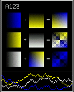 The above figure shows the physical
layout of the positions and it shows how the chosen color ramps add
together. Choosing color ramps that do not blend correctly will result
in blockiness in the sum of the color equations (see the example to the
right). This would be bad, and checking the color mixing blocks for
damage will prevent mixing problems in the spectrogram window at different
amplitude (dB) levels. The black color mixing box can also be used
as a visual status showing which channels are enabled, and their location
in the spectral display.
The above figure shows the physical
layout of the positions and it shows how the chosen color ramps add
together. Choosing color ramps that do not blend correctly will result
in blockiness in the sum of the color equations (see the example to the
right). This would be bad, and checking the color mixing blocks for
damage will prevent mixing problems in the spectrogram window at different
amplitude (dB) levels. The black color mixing box can also be used
as a visual status showing which channels are enabled, and their location
in the spectral display.
|