baudline solution - sine distortion measurements

Abstract

Sine Distortion Measurements
E. Olson, April 19 2005

Develop an experimental technique for determining SNR, THD, SINAD, ENOB, and SFDR distortion measurements from a full duplex black box DUT by using a clean sine wave as the stimulus signal. The distortion measurements are valuable performance metrics for evaluating signal quality and loss. The effects of frequency, FFT size, windowing function, gain, tone generator shapes, and channel operations will be explored. The goal is to create a reliable and repeatable procedure for quickly and accurately measuring signal quality.

Procedure

Use the baudline signal analyzer to generate the sine wave source, capture the input signal, and calculate the distortion measurements. The following describes the theory and procedure needed to accomplish full duplex black box testing.

black box
Treat the Device Under Test (DUT) as an unknown black box that cannot be opened and inspected. The gears, levers, and circuitry inside are a mystery. The only way information about the DUT's working internals can be learned is by probing with an input stimulus and then measuring the output characterization signal. It is a basic case of cause and effect. Standard black box testing consists of three elements:

test signal generator (source)
black box (DUT)
signal analysis tool (sink)

signal source
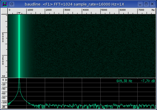
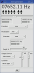
The sine function in the Tone Generator is used as the stimulus signal. The sine wave is an ideal test signal because it is spectrally pure and it consists of only a single peak in the frequency domain. A clean sine wave has no harmonics and any channel distortions or errors that differ from the main fundamental frequency peak will be easily distinguishable.

The choice of fundamental frequency is important because several distortion measurements take advantage of harmonic spacing. Since many different sample rates may be tested it is critical that the fundamental frequency move in proportion to the changing Nyquist frequency limits. The idea is to hold harmonic spacing and FFT bin position constant for all sample rates. This way distortion measurements from different sample rates can be fairly compared.

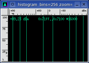
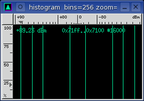Frequencies that are an integer multiple of the sample rate have the unique trait of being highly repetitive. They consist of just a couple sample values that repeat over and over. This can be seen and measured with the Histogram window (see the image on the right). Only 8 histogram bins are used in this example. The problem is that this sparse distribution behavior doesn't exercise all of the ADC and DAC bits. It is possible that a serious problem could be masked.

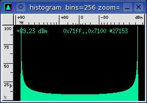
To solve the potential repetitive bits problem a small fractional offset is added to the fundamental test frequency. This offset reduces the sample clusters and results in a more evenly populated histogram (see the image on the right). The new flatter sample distribution will highlight any sticky bits or gross requantization errors. Strange features in the Histogram domain usually manifest themselves as noise floor shapes or weak spurious peaks in the spectral domain.

The following formula satisfies the above constraints:

fundamental Hz = sample rate / 26.5 + .1;

`rate`	`Hz`
`4000`	`151.04`
`5510`	`208.02`
`8000`	`301.99`
`11025`	`416.14`
`12000`	`452.93`
`16000`	`603.87`
`22050`	`832.18`
`24000`	`905.76`
`32000`	`1207.65`
`44100`	`1664.25`
`48000`	`1811.42`
`64000`	`2415.19`

loopback setup
The goal is to create a robust procedure for testing and measuring the ADC and DAC quality of a computer sound card. Using a minimal amount of external equipment is also a bonus. To accomplish this task the black box testing paradigm is flipped by making the black box test itself. The black box now becomes the cable. Or as is depicted in the picture on the right, the black box now becomes baudline! With baudline there are four possible loopback modes:

external cable
internal "volume" mixer channel
digital tone generator loopback option
half duplex operation for special cases

The first three are proper full duplex modes where the sound card's input is connected to it's output. For half duplex an external function generator is required (this could be a second sound card running baudline). The half duplex mode is important for two reasons; some older sound cards only operate at half duplex, and with some sound cards the full duplex performance is different than the half duplex performance.

The majority of this experiment will use the digital tone generator loopback option which is basically a virtual cable. It is a 100% digital path and it will define the baseline performance level. The lessons learned here will be generic in nature and applicable to the standard definition of black box testing.

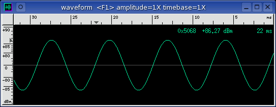
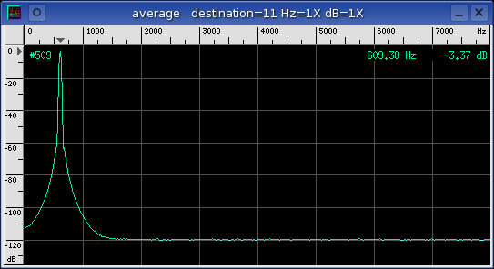
capture sink
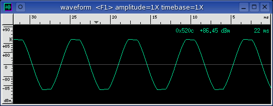
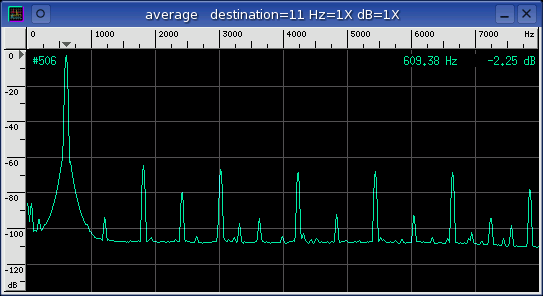
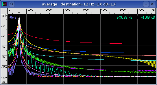
The above Waveform and Average windows show a sine wave signal source that has been looped back and captured by baudline in the record mode. The sine waveform is well defined and it is -3 dB away from the 16-bit max saturation clipping point. The average spectrum has a strong fundamental peak with no harmonics and a very flat noise floor. This is a good example of what a clean and correctly adjusted setup should look like.

distortion measurements
Distortions and errors can manifest themselves as harmonics, side lobes, modulations, spurious peaks, or other forms of noise. They can be linear or nonlinear in nature but the net effect is the same and that is signal corruption.

Baudline has a set of built in distortion measurements that will automatically calculate SNR, THD, SINAD, ENOB, and SFDR. The Signal to Noise Ratio (SNR) is useful for measuring the characterization of the noise floor. Total Harmonic Distortion (THD) is a measure of nonlinearity. Signal to Noise and Distortion Ratio (SINAD) is a measure of signal purity. Effective Number of Bits (ENOB) is calculated from SINAD and describes the quality of an ADC in terms of bits. Spurious Free Dynamic Range (SFDR) is a measure of dynamic range which is the ratio of the input signal to the strongest non signal element (spurious peak). Each distortion measurement has it's uses but the two most valuable are THD and ENOB.

optimal gain settings
The input and output mixer gain settings can have a dramatic effect on the distortion measurements. Simply adjusting the gains so that the test signal is just a fraction of a dB away from the point of clipping is not sufficient. With systematic tweaking an extra bit or two of ENOB can be achieved. Note that the optimal gain settings will vary from device to device because of different amplifier nonlinearities.

Below is an example of amplifier clipping and the severe harmonic distortion it can cause.

The technique for finding the optimal gain settings varies from card to card but the common plan is to adjust the input and output mixer gain controls so that the ENOB value is maximized. A good algorithmic procedure for gain convergence is:

initial state
1. Set digital tone generator gain to 0 dB.
2. Set the input mixer gain to the lowest value that does not completely attenuate the recording signal.
3. Set the output mixer gain to the maximum value that does not have gross harmonic distortion (see above picture).
4. Slowly increase the input mixer gain until gross distortion sets in then back off by one click.
5. This might be the best ENOB setting.
search analog mixer
1. Decrease the output mixer gain by one click. (Down arrow key)
2. Increase the input mixer gain by one click. (Up arrow key)
3. If the ENOB value is better then repeat, if not then go back to previous setting and continue with the next search.
search digital gain
1. Decrease the digital tone generator gain by 1 dB.
2. Alternately increase the input and/or output mixer gains by one click.
3. If the ENOB value is better then repeat, if not then go back to previous setting and exit.
Choose the gain settings that result in the best ENOB value.

goals
The important experimental questions are:

What distortions are made to the known signal input?
What does this tell us about the inner workings of the black box?
How can we optimize the input signal parameters for the best performance?
How accurate are the measurements?

Data

Explore variable space. Measure the effect of changing a single test parameter while holding all the other parameters constant. This way each parameter can be studied individually. The following "variations on a variable" experiments will be conducted:

digital gain
fft size
frequency
windowing function
generator function
channel operation
digital loopback vs. cards

baudline setup
The tone generator loopback option in the Input Devices window is enabled for a clean 100% digital loopback. This is baudline's baseline level of performance. A DUT such as a sound card cannot have performance greater than this baseline unless it employs active noise reduction.

Except for the variable under test and unless specifically noted; all of the "variable" tests use these baudline settings and methods:

input devices
- 16000 sample rate
- decimate by none
- tone generator loopback enabled
tone generator
- main frequency 603.87 Hz
- sine wave function
- modulation OFF
- digital gain 0 dB
0.71 overlap sqrt(%)
1024 point FFT
Blackman window
spectrum slices collected in Average window for #500 count
distortion measurements
- source set to "average"
- fundamental rule set to "use primary Hz"

variable digital gain
Explore the effect of signal amplitude. Vary the digital gain control in the Tone Generator window. How do the distortion measurements change as the gain decreases?

`gain`	`SNR`	`THD`	`SINAD`	`ENOB`	`SFDR`
`0 dB`	`+96.60 dB`	`-104.59 dB`	`+95.96 dB`	`+15.646 bits`	`+111.90 dB`
`-6 dB`	`+90.68 dB`	`-97.44 dB`	`+89.85 dB`	`+14.632 bits`	`+110.56 dB`
`-12 dB`	`+84.77 dB`	`-91.04 dB`	`+83.85 dB`	`+13.635 bits`	`+102.95 dB`
`-18 dB`	`+78.68 dB`	`-85.03 dB`	`+77.77 dB`	`+12.625 bits`	`+96.83 dB`
`-24 dB`	`+72.59 dB`	`-78.58 dB`	`+71.62 dB`	`+11.603 bits`	`+87.23 dB`
`-30 dB`	`+66.85 dB`	`-71.51 dB`	`+65.58 dB`	`+10.599 bits`	`+84.80 dB`
`-36 dB`	`+60.32 dB`	`-66.94 dB`	`+59.45 dB`	`+9.585 bits`	`+77.06 dB`
`-42 dB`	`+54.28 dB`	`-60.86 dB`	`+53.42 dB`	`+8.580 bits`	`+69.56 dB`
`-48 dB`	`+47.99 dB`	`-55.70 dB`	`+47.31 dB`	`+7.566 bits`	`+63.99 dB`
`-54 dB`	`+41.95 dB`	`-49.89 dB`	`+41.30 dB`	`+6.568 bits`	`+57.40 dB`
`-60 dB`	`+36.22 dB`	`-41.96 dB`	`+35.20 dB`	`+5.553 bits`	`+51.46 dB`
`-66 dB`	`+29.86 dB`	`-37.44 dB`	`+29.16 dB`	`+4.551 bits`	`+46.89 dB`
`-72 dB`	`+24.28 dB`	`-30.73 dB`	`+23.40 dB`	`+3.594 bits`	`+40.12 dB`
`-78 dB`	`+18.28 dB`	`-26.26 dB`	`+17.64 dB`	`+2.638 bits`	`+36.71 dB`
`-84 dB`	`+12.66 dB`	`-19.99 dB`	`+11.92 dB`	`+1.687 bits`	`+27.81 dB`
`-90 dB`	`+7.05 dB`	`-14.30 dB`	`+6.30 dB`	`+0.754 bits`	`+22.74 dB`
`-96 dB`	`-0.59 dB`	`-6.63 dB`	`+1.34 dB`	`-0.515 bits`	`+15.17 dB`
`-102 dB`	`-4.68 dB`	`-1.74 dB`	`-5.57 dB`	`-1.218 bits`	`+12.80 dB`
`-108 dB`	`-7.59 dB`	`+0.05 dB`	`-8.29 dB`	`-1.670 bits`	`+8.93 dB`
`-114 dB`	`-9.46 dB`	`+3.03 dB`	`-10.35 dB`	`+2.012 bits`	`+5.32 dB`
`-120 dB`	`-11.40 dB`	`+4.96 dB`	`-12.29 dB`	`-2.334 bits`	`+4.11 dB`
`-126 dB`	`-13.91 dB`	`+7.07 dB`	`-14.73 dB`	`-2.739 bits`	`+2.11 dB`
`-132 dB`	`-13.71 dB`	`+6.01 dB`	`-14.39 dB`	`-2.682 bits`	`+4.73 dB`

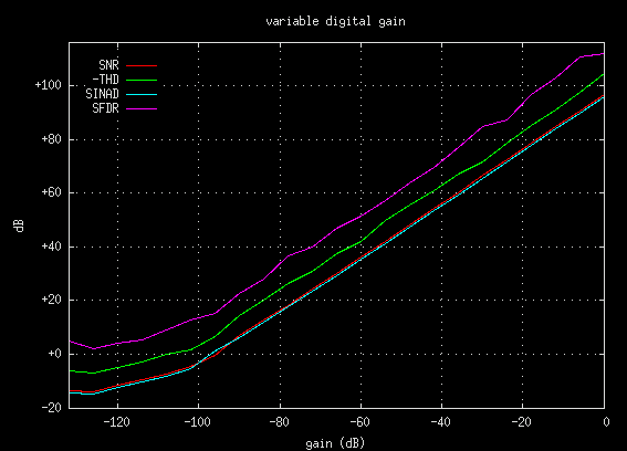
The plot below shows that the gain (dB) influence on the distortion metrics is fairly linear from 0 dB to about the -100 dB point. Note that -THD is inverted so that it matches the range of the dB axis. Reducing the output gain by 6 dB results in a 6 dB change of the distortion metrics. Below the -100 dB point the signal is very weak and a combination of dither and low bit effects take over.

variable FFT size
Explore the effect of FFT size. Vary the transform size setting. Other than the effects of frequency discrimination and resolution, are there any benefits to using a larger FFT size?

`FFT size`	`SNR`	`THD`	`SINAD`	`ENOB`	`SFDR`
`128`	`+107.23 dB`	`-99.53 dB`	`+98.85 dB`	`+16.126 bits`	`+103.19 dB`
`256`	`+103.18 dB`	`-99.32 dB`	`+97.83 dB`	`+15.956 bits`	`+108.89 dB`
`512`	`+98.08 dB`	`-101.98 dB`	`+96.60 dB`	`+15.752 bits`	`+115.35 dB`
`1024`	`+96.97 dB`	`-103.09 dB`	`+96.02 dB`	`+15.656 bits`	`+113.76 dB`
`2048`	`+96.12 dB`	`-105.73 dB`	`+95.67 dB`	`+15.598 bits`	`+114.73 dB`
`4096`	`+95.60 dB`	`-108.34 dB`	`+95.38 dB`	`+15.549 bits`	`+116.36 dB`
`8192`	`+95.33 dB`	`-111.90 dB`	`+95.24 dB`	`+15.526 bits`	`+122.00 dB`
`16384`	`+95.22 dB`	`-114.61 dB`	`+95.17 dB`	`+15.514 bits`	`+121.52 dB`
`32768`	`+95.16 dB`	`-117.47 dB`	`+95.14 dB`	`+15.510 bits`	`+127.30 dB`
`65536`	`+95.12 dB`	`-121.32 dB`	`+95.11 dB`	`+15.505 bits`	`+126.84 dB`

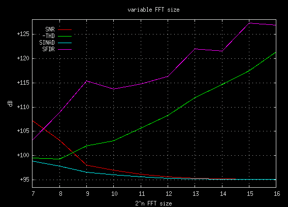
The plot below shows the FFT size (2^n) influence on the distortion metrics. Note that -THD is inverted so that it matches the range of the dB axis. The SNR and SINAD curves look like they are exponentially converging to a +95 dB value as the FFT size increases. If the first two FFT sizes (128 and 256) are ignored then the THD and SFDR behavior becomes fairly predictable. In fact, THD is decreasing 3 dB for each FFT size doubling while SFDR is increasing by 2 dB per doubling. This steady change can be explained as being due to FFT gain (which is like decimation gain).

Because of the mysterious nonlinear bottom end effect mentioned above, FFT sizes greater than 512 points are recommended when making distortion measurements. Depending on the particular signal distortions, a much larger FFT size could be beneficial. For example: a high frequency mega sample rate signal that has been modulated with 60 Hz bleed in. A small FFT will not have the frequency resolution/discrimination to pull out the 60 Hz AM bands, the fundamental will look like a nice clean lobe and the modulation distortion will remain hidden.

The most important point learned from this experiment is that when working with distortion measurements it is imperative to know the FFT size. Since THD and SFDR values scale linearly with FFT size (2^n), not knowing the FFT size renders any distortion specifications meaningless.

variable frequency
Explore different fundamental stimulus frequencies. Vary the main frequency control in the Tone Generator window. Which distortion measurements are a function of input frequency?

`frequency`	`SNR`	`THD`	`SINAD`	`ENOB`	`SFDR`
`500 Hz`	`+96.86 dB`	`-103.06 dB`	`+95.92 dB`	`+15.640 bits`	`+118.01 dB`
`1000 Hz`	`+95.28 dB`	`-104.31 dB`	`+94.77 dB`	`+15.449 bits`	`+111.77 dB`
`2000 Hz`	`+94.23 dB`	`-108.55 dB`	`+94.08 dB`	`+15.333 bits`	`+110.58 dB`
`3000 Hz`	`+94.82 dB`	`-111.34 dB`	`+94.72 dB`	`+15.441 bits`	`+112.97 dB`
`4000 Hz`	`+93.96 dB`	`-inf.00 dB`	`+93.96 dB`	`+15.313 bits`	`+109.64 dB`
`5000 Hz`	`+94.75 dB`	`-inf.00 dB`	`+94.75 dB`	`+15.444 bits`	`+110.57 dB`
`6000 Hz`	`+94.15 dB`	`-inf.00 dB`	`+94.15 dB`	`+15.345 bits`	`+108.98 dB`
`7000 Hz`	`+95.70 dB`	`-inf.00 dB`	`+95.70 dB`	`+15.603 bits`	`+114.74 dB`

The above data hints at a deeper complex behavior but it lacks the necessary granularity to fully observe it. So in an effort to improve the resolution this variable frequency test was re-run with a slow sine sweep. Data points were collected with the -debugmeasure command line option and the plot below shows this more detailed view. Note that -THD is inverted so that it matches the range of the dB axis.

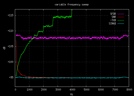
A number of interesting relationships are present in the above plot. Three particularly unusual behaviors will be discussed below:

SNR and SINAD convergence
The SNR measurement has an exponential decay towards SINAD until it reaches half the Nyquist frequency (4000 Hz) where it converges. This follows the numeric theory of harmonics; the integer number of harmonics is inversely proportional to frequency.
THD stairsteps
The -THD plot begins as an exponential increase, then it transcends into eight distinct energy levels, and finally it becomes undefined as +infinity. The low end exponential increase follows the same logic that the SNR explanation used; the integer number of harmonics is inversely proportional to the frequency. Then at about 800 Hz the first of eight distinct energy levels appear. These quanta exhibit a successive doubling of frequency width which follows the general shape of the exponential curve. Their presence is explained by the fact that the number of harmonics is an integer. To understand this phenomena better try experimenting with the harmonic helper bars.
Left and right frequency bumps.
The SNR, SINAD, and SFDR measurements exhibit slight bumps at the edges of the frequency spectrum. This is caused when the finite width windowing lobes hit the left or right spectral edges. A theoretical zero width lobe would not do this.

The important lesson here is that frequency position within the spectrum can have an important effect on the distortion measurements. Just like with the FFT size experiment, for the THD measurement to be valid the frequency of the fundamental must be declared.

variable windowing function
Explore the effect of FFT windowing. Vary the windowing function in the Windowing window. Which windowing functions are most appropriate for making distortion measurements?

`function`	`SNR`	`THD`	`SINAD`	`ENOB`	`SFDR`
`square`	`+55.10 dB`	`-inf.00 dB`	`+55.10 dB`	`+8.859 bits`	`+55.10 dB`
`Parzen`	`+89.78 dB`	`-97.24 dB`	`+89.06 dB`	`+14.500 bits`	`+101.30 dB`
`Welch`	`+85.23 dB`	`-89.01 dB`	`+83.71 dB`	`+13.611 bits`	`+90.28 dB`
`Hanning`	`+96.95 dB`	`-104.19 dB`	`+96.20 dB`	`+15.686 bits`	`+118.32 dB`
`Hamming`	`+35.84 dB`	`-67.00 dB`	`+35.84 dB`	`+5.660 bits`	`+35.84 dB`
`Blackman`	`+96.94 dB`	`-102.94 dB`	`+95.97 dB`	`+15.647 bits`	`+113.57 dB`
`Kaiser b6`	`+55.74 dB`	`-58.11 dB`	`+53.75 dB`	`+8.636 bits`	`+53.81 dB`
`Kaiser b11`	`+95.20 dB`	`-101.32 dB`	`+94.25 dB`	`+15.363 bits`	`+105.83 dB`
`Kaiser b15`	`+96.83 dB`	`-102.42 dB`	`+95.77 dB`	`+15.615 bits`	`+108.10 dB`
`Gaussian b6`	`+96.40 dB`	`-101.73 dB`	`+95.28 dB`	`+15.534 bits`	`+104.85 dB`
`Gaussian b11`	`+97.71 dB`	`-101.19 dB`	`+96.10 dB`	`+15.669 bits`	`+102.88 dB`
`Cauchy b6`	`+74.58 dB`	`-71.07 dB`	`+69.47 dB`	`+11.246 bits`	`+71.07 dB`
`Poisson b6`	`+88.16 dB`	`-inf.00 dB`	`+88.16 dB`	`+14.351 bits`	`+91.06 dB`
`Tukey b6`	`+25.90 dB`	`-65.34 dB`	`+25.90 dB`	`+4.01 bits`	`+26.55 dB`

The above ENOB values show that most windowing functions are not appropriate for making accurate distortion measurements. The Hanning and Blackman windows are recommended. The Kaiser window with a beta greater than 11.00 and the Gaussian window with a beta greater than 5.00 will also work. Caution should be exercised with large beta's because the lobe width increases to a point that frequency resolution is severely hampered.

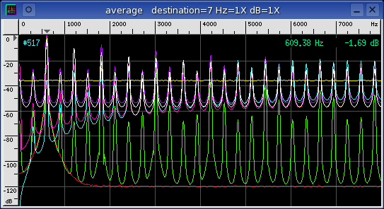
The Average window below is a spectrum plot of all the different Windowing functions.

legend (from bottom up)

magenta - Blackman
orange - Hanning
lavender - Kaiser b11
pink - Gaussian b6
...
red - square

variable generator function
Explore the effect of different stimulus functions. Vary the fundamental function in the Tone Generator window. Is sine the only function that is appropriate for making distortion measurements?

`function`	`SNR`	`THD`	`SINAD`	`ENOB`	`SFDR`
`sine`	`+97.02 dB`	`-102.88 dB`	`+96.02 dB`	`+15.656 bits`	`+110.40 dB`
`triangle`	`+42.35 dB`	`-18.35 dB`	`+18.33 dB`	`+2.753 bits`	`+19.08 dB`
`square`	`+15.50 dB`	`-6.88 dB`	`+6.32 dB`	`+0.757 bits`	`+9.532 dB`
`ramp up`	`+12.35 dB`	`-2.33 dB`	`+1.92 dB`	`+0.026 bits`	`+6.00 dB`
`ramp down`	`+12.35 dB`	`-2.33 dB`	`+1.92 dB`	`+0.026 bits`	`+6.00 dB`
`unit impulse`	`-4.88 dB`	`+9.78 dB`	`-11.00 dB`	`-2.119 bits`	`+1.01 dB`
`doublet impulse`	`-21.06 dB`	`+25.40 dB`	`-26.76 dB`	`-4.737 bits`	`-16.25 dB`
`WGN`	`+15.84 dB`	`+7.94 dB`	`-16.49 dB`	`-3.032 bits`	`+1.88 dB`

For unit impulse, doublet impulse, and WGN (white Gaussian noise) the fundamental rule "max in Hz range" was used with a 578 Hz to 640 Hz frequency range. This was because all three signal sources had incorrect fundamentals due to their definition.

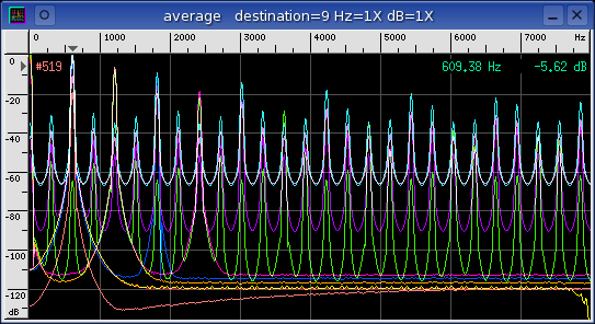
The Average window below is a spectrum plot of all the different Tone Generator functions. None of the functions are suitable as a stimulus for distortion measurements expect for the standard sine wave (red). The triangle function (green) is a good demonstration of what a severely distorted signal would look like with an ENOB of 2.7 bits.

variable channel operation
Explore the effect of different mathematical operations. Vary the operations in the Input Channel Mapping window. How do the distortion results compare with the data that was collected in the stimulus function experiment above?

`operation`	`SNR`	`THD`	`SINAD`	`ENOB`	`SFDR`
`none`	`+96.83 dB`	`-103.70 dB`	`+96.02 dB`	`+15.655 bits`	`+113.92 dB`
`\| x \|`	`-64.85 dB`	`+56.55 dB`	`-65.45 dB`	`-11.163 bits`	`-64.85 dB`
`sqrt`	`+32.23 dB`	`-15.60 dB`	`+15.51 dB`	`+2.283 bits`	`+16.90 dB`
`x^2`	`-107.94 dB`	`+42.80 dB`	`-107.94 dB`	`-18.221 bits`	`-106.75 dB`
`x^3`	`+89.44 dB`	`-9.54 dB`	`+9.54 dB`	`+1.292 bits`	`+9.65 dB`
`x^4`	`-104.02 dB`	`+83.09 dB`	`-104.05 dB`	`-17.576 bits`	`-102.02 dB`
`log`	`+19.36 dB`	`-8.56 dB`	`+8.21 dB`	`+1.071 bits`	`+10.77 dB`
`clip`	`+15.50 dB`	`-6.88 dB`	`+6.32 dB`	`+0.757 bits`	`+9.53 dB`
`delta`	`+80.41 dB`	`-87.16 dB`	`+79.58 dB`	`+12.925 bits`	`+92.77 dB`
`Hilbert`	`+96.65 dB`	`-103.20 dB`	`+95.78 dB`	`+15.616 bits`	`+112.60 dB`

The fundamental rule "max in Hz range" was used with a 578 Hz to 640 Hz frequency range for problem operations like absolute value, x^2, and x^4. Notice that the sign of the distortion measurements has flipped for the "problem operations." This signifies that there is more noise and distortion than there is signal.

The Average window below is a spectrum plot of all the different channel operations. Many of the spectrum plots look similar to some of the Tone Generator functions in the previous experiment. Of particular interest is the delta operation (orange) which has a lower noise floor than the default "none" operation.

digital loopback vs. cards
Measure the distortion values of a couple different sound card audio devices. Compare the results with the baseline digital tone loopback (with and without dither).

`device`	`SNR`	`THD`	`SINAD`	`ENOB`	`SFDR`
`digital`	`+96.80 dB`	`-103.55 dB`	`+95.96 dB`	`+15.647 bits`	`+112.90 dB`
`digital -nodither`	`+99.76 dB`	`-107.55 dB`	`+99.09 dB`	`+16.166 bits`	`+115.44 dB`
`SBLive EMU10K1`	`+73.86 dB`	`-80.84 dB`	`+73.07 dB`	`+11.844 bits`	`+73.97 dB`
`CS4236B (0 dB)`	`+76.01 dB`	`-57.97 dB`	`+57.90 dB`	`+9.324 bits`	`+64.68 dB`
`CS4236B (-1 dB)`	`+75.50 dB`	`-74.09 dB`	`+71.73 dB`	`+11.621 bits`	`+74.86 dB`
`iMic v0.06`	`+74.61 dB`	`-92.29 dB`	`+74.54 dB`	`+12.088 bits`	`+74.77 dB`
`iMic v3.00`	`+71.30 dB`	`-76.78 dB`	`+70.22 dB`	`+11.370 bits`	`+72.04 dB`

The Sound Blaster Live! card has an incredibly complicated mixer. Finding the optimal mixer settings was a very complex process. In fact a separate mixer program had to be used to disable some of the SBLive's more exotic defaults. After this was done and the card was dialed in some fairly respectable distortion measurement were possible.

A Crystal CS4236B audio chip (on motherboard) was tested at the Tone Generators 0 dB and -1 dB digital gain levels. The lower -1 dB digital gain level resulted in about a 14 dB improvement with both the THD and SINAD measurements. This discrepancy indicates a MSB or a numeric overflow problem with the CS4236B. With the CS4236B chip it is best to avoid loud signals that use all of the 16 bit dynamic range.

For a more thorough coverage of this topic see the sound card comparison application note.

Conclusion

After exploring variable space in these 7 experiments it became very obvious that both testing strategy and baudline parameter settings play a critical role in the reliability and repeatability of DUT distortion measurement analysis. Some parameter settings are more appropriate than others for DUT testing. Also any slight parameter variation between tests can lead to significant differences. It is recommended to define a group of baudline parameter settings, possibly with the -session command, and use those preset defaults for all DUT testing.

Another important observation was the effect that FFT size and test frequency have on the absolute reporting of distortion measurements. The SNR, THD, and SFDR measurements are tightly coupled to both FFT size and test frequency while the SINAD and ENOB measurements have a looser coupling. In fact, THD measurements can vary by as much as 40 dB simply by changing both the FFT size and the test frequency parameters. For noise and distortion measurements to be valid they must be accompanied by the FFT size and test frequency values.

The final observation is a tip on how to get the best audio playback quality from a sound card. Setting the output mixer gain to maximum caused significant distortion with all of the sound cards tested. This distortion goes away when the output mixer gain is set to approximately 75%. Backing off slightly on the mixer gain will improve quality.